39 excel chart only show certain data labels

Excel 2016 Chart Data Labels Always Empty - Stack Overflow I have several bar charts, all configured to show Data Labels. The data labels object box is showing (I can also apply Fill and Border colors to it). However, this object is always EMPTY. Regardless of what I tick to show (e.g. Values, Values from Cells, Series Name, etc...) - it is always empty, with the minimum (shrunk) width (as it should ... Individually Formatted Category Axis Labels - Peltier Tech Format the category axis (horizontal axis) so it has no labels. Add data labels to the the dummy series. Use the Below position and Category Names option. Format the dummy series so it has no marker and no line. To format an individual label, you need to single click once to select the set of labels, then single click again to select the ...

How to hide zero data labels in chart in Excel? - ExtendOffice Sometimes, you may add data labels in chart for making the data value more clearly and directly in Excel. But in some cases, there are zero data labels in the chart, and you may want to hide these zero data labels. Here I will tell you a quick way to hide the zero data labels in Excel at once. Hide zero data labels in chart

Excel chart only show certain data labels

Display every "n" th data label in graphs - Microsoft Community you can use a free tool created by Rob Bovey, called the XY Chart Labeler. With this tool you can assign a range of cells to be the labels for chart series, instead of the Excel defaults. Using a formula, you can have a text show up in every nth cell and then use that range with the XY Chart Labeler to display as the series label. Solved: Show data label only to one line - Power BI Remove the legend and the current measure from the line chart. 3. Add all of the measures to the line chart. 4. Then Data Labels will have the Customize Series option. Message 4 of 8 11,827 Views 2 Reply Add a DATA LABEL to ONE POINT on a chart in Excel Steps shown in the video above: Click on the chart line to add the data point to. All the data points will be highlighted. Click again on the single point that you want to add a data label to. Right-click and select ' Add data label ' This is the key step! Right-click again on the data point itself (not the label) and select ' Format data label '.

Excel chart only show certain data labels. Dynamically Label Excel Chart Series Lines - My Online Training Hub Step 1: Duplicate the Series. The first trick here is that we have 2 series for each region; one for the line and one for the label, as you can see in the table below: Select columns B:J and insert a line chart (do not include column A). To modify the axis so the Year and Month labels are nested; right-click the chart > Select Data > Edit the ... Add data labels to chart but only for most recent and oldest value For a new thread (1st post), scroll to Manage Attachments, otherwise scroll down to GO ADVANCED, click, and then scroll down to MANAGE ATTACHMENTS and click again. Now follow the instructions at the top of that screen. New Notice for experts and gurus: Excel tutorial: Dynamic min and max data labels To make the formula easy to read and enter, I'll name the sales numbers "amounts". The formula I need is: =IF (C5=MAX (amounts), C5,"") When I copy this formula down the column, only the maximum value is returned. And back in the chart, we now have a data label that shows maximum value. Now I need to extend the formula to handle the minimum value. How to add data labels from different column in an Excel chart? Click any data label to select all data labels, and then click the specified data label to select it only in the chart. 3. Go to the formula bar, type =, select the corresponding cell in the different column, and press the Enter key. See screenshot: 4. Repeat the above 2 - 3 steps to add data labels from the different column for other data points.

Chart: only show legend elements with values - MrExcel Message Board However, each graph only needs 3-4 elements out of the 20 legend entries in the graph. Thanks in advance! Not sure how your data is arrange/organised, but you could filter data to show only 'Greater than or equal to' 0 (zero), such would hide the rows with NA () and would display a chart with only data with value. Excel chart not showing all data selected - Microsoft Community Double-click any of the dates along the x-axis, or the x-axis itself. In the Format Axis taskpane, look at the Minimum and Maximum. If you see Reset next to the box, click it to make the bound automatic (it should read Auto after that) --- Kind regards, HansV Report abuse 76 people found this reply helpful · Add or remove data labels in a chart - support.microsoft.com Click the data series or chart. To label one data point, after clicking the series, click that data point. In the upper right corner, next to the chart, click Add Chart Element > Data Labels. To change the location, click the arrow, and choose an option. If you want to show your data label inside a text bubble shape, click Data Callout. Custom Chart Data Labels In Excel With Formulas Select the chart label you want to change. In the formula-bar hit = (equals), select the cell reference containing your chart label's data. In this case, the first label is in cell E2. Finally, repeat for all your chart laebls. If you are looking for a way to add custom data labels on your Excel chart, then this blog post is perfect for you.

Find, label and highlight a certain data point in Excel scatter graph ... Select the Data Labels box and choose where to position the label. By default, Excel shows one numeric value for the label, y value in our case. To display both x and y values, right-click the label, click Format Data Labels…, select the X Value and Y value boxes, and set the Separator of your choosing: Label the data point by name How to Use Cell Values for Excel Chart Labels Select the chart, choose the "Chart Elements" option, click the "Data Labels" arrow, and then "More Options." Uncheck the "Value" box and check the "Value From Cells" box. Select cells C2:C6 to use for the data label range and then click the "OK" button. The values from these cells are now used for the chart data labels. charts - Excel, giving data labels to only the top/bottom X% values ... 1) Create a data set next to your original series column with only the values you want labels for (again, this can be formula driven to only select the top / bottom n values). See column D below. 2) Add this data series to the chart and show the data labels. 3) Set the line color to No Line, so that it does not appear! 4) Volia! See Below! Share How to Conditionally Show or Hide Charts - Excel Chart Templates ... In a complicated Excel 2003 chart, which has two 4-point area chart series to highlight a background range, and an XY series with custom markers (pasted shapes) and more then 4 points, only the first four points appear with their custom markers, though the code that applies the markers does not fail, and the data labels for the marker-less ...

Learn SEO The Ultimate Guide For SEO Beginners 2020 - Your Optimized Solutions

Highlight a Specific Data Label in an Excel Chart - Peltier Tech * right click on the series, choose Change Series Chart Type from the pop up menu, and select the desired chart type. Add data labels to each line chart* (left), then format them as desired (right). * right click on the series, choose Add Data Labels from the pop up menu. Finally format the two line chart series so they use no line and no marker.

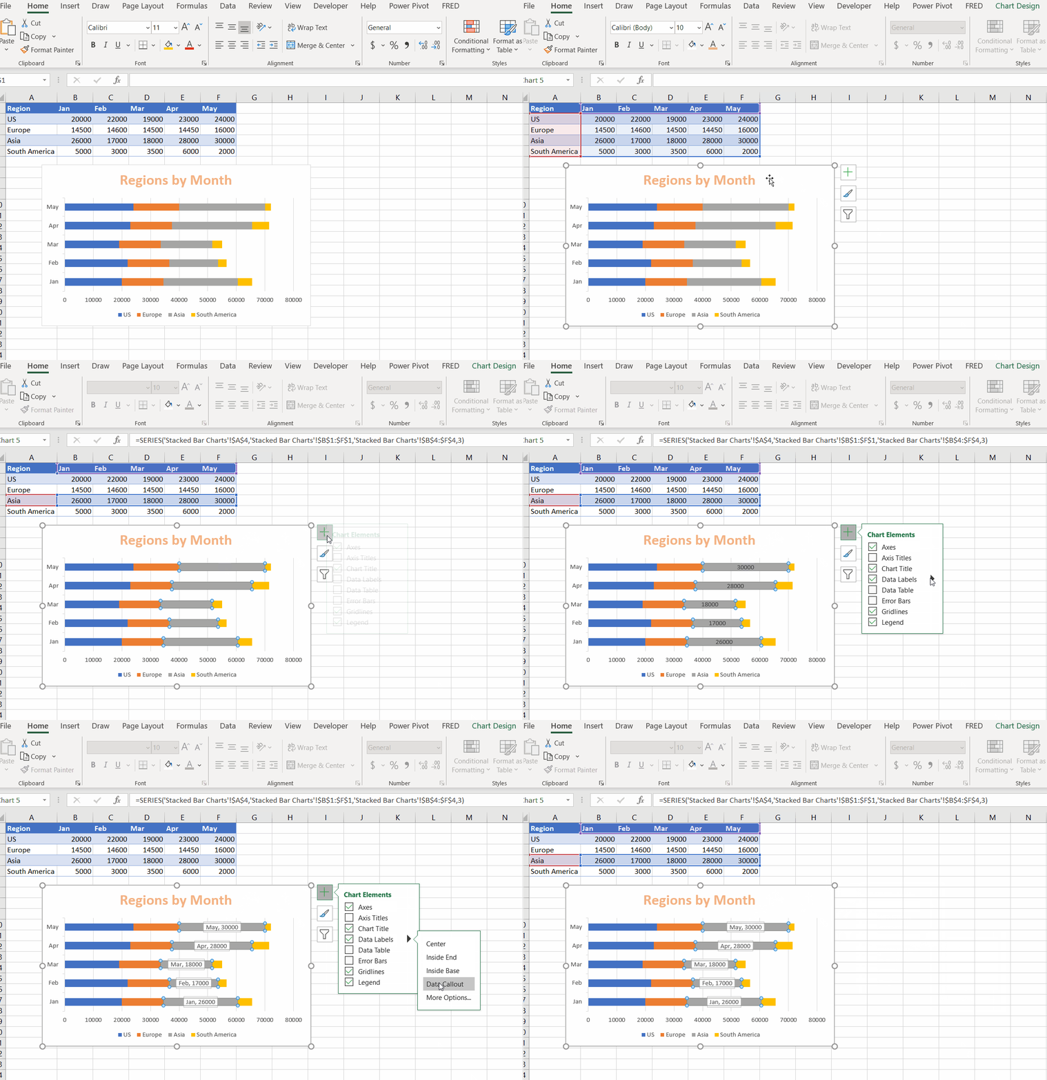
Excel Bar Charts - Clustered, Stacked - Template - Automate Excel

Change the format of data labels in a chart To get there, after adding your data labels, select the data label to format, and then click Chart Elements > Data Labels > More Options. To go to the appropriate area, click one of the four icons ( Fill & Line, Effects, Size & Properties ( Layout & Properties in Outlook or Word), or Label Options) shown here.

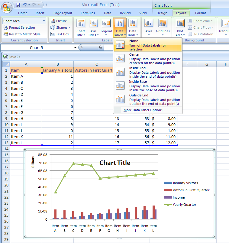
Change Chart Data Labels : Chart Data « Chart « Microsoft Office Excel 2007 Tutorial

How to Change Excel Chart Data Labels to Custom Values? This will select "all" data labels. Now click once again. At this point excel will select only one data label. Go to Formula bar, press = and point to the cell where the data label for that chart data point is defined. Repeat the process for all other data labels, one after another. See the screencast. Points to note:

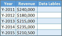
How To Use Dynamic Data Labels To Create Interactive Excel Charts

Only Label Specific Dates in Excel Chart Axis - YouTube Date axes can get cluttered when your data spans a large date range. Use this easy technique to only label specific dates.Download the Excel file here: https...

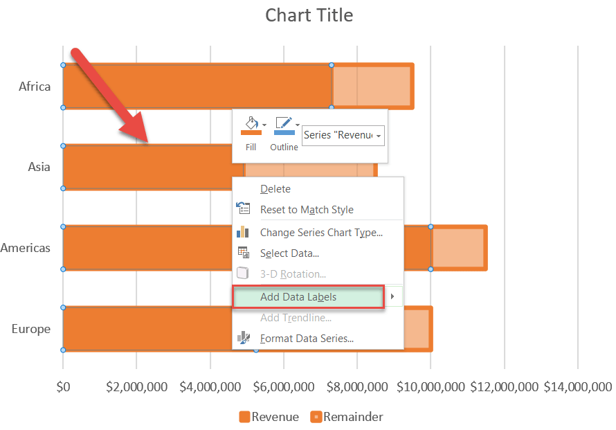
How to Create Progress Charts (Bar and Circle) in Excel - Automate Excel

Hiding data labels for some, not all values in a series Here's a good challenge for you. I can't figure it out, and I believe it's a limitation of Excel. I have a bar graph with several data series. I know how to show the data labels for every data point in a given series. But I'm looking to show the data label for only some data points in a given series -- i.e. non-zero valued data points.

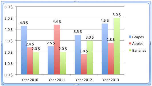
Format Number Options for Chart Data Labels in Excel 2011 for Mac

Hiding certain series in an excel data table (but displaying those ... Create the chart with all 3 series (i.e. the three series and the total) as a stacked chart. Then right-click on the 'Total' series, select Chart Type and change it to a line chart. Lastly, double-click the line and format it to have no line or markers. It should then be included in the data table, but not be visible in the chart. Report abuse

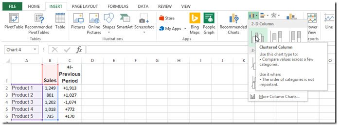
How-to Use Data Labels from a Range in an Excel Chart - Excel Dashboard Templates

How to Only Show Selected Data Points in an Excel Chart Download Free Sample Dashboard Files here: on how to show or hide specific data points i...

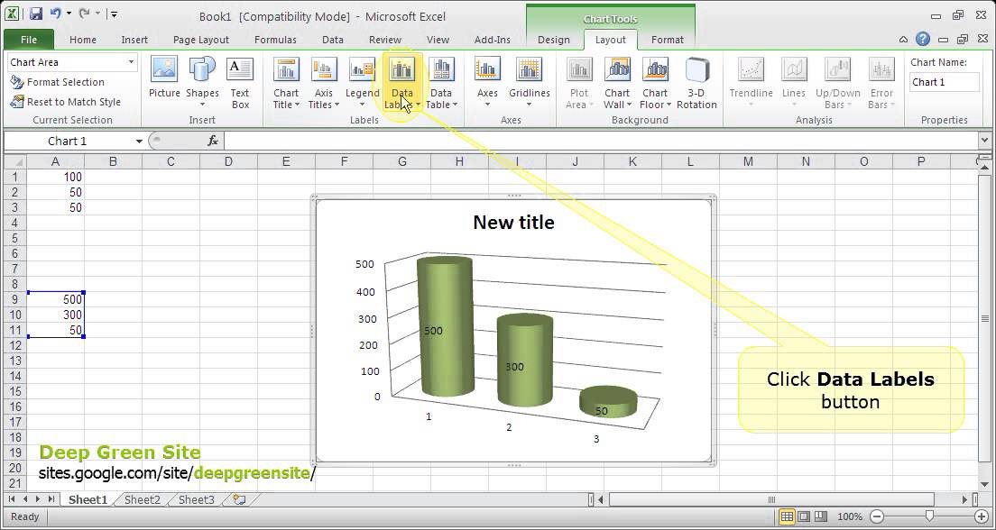
MS Excel 2010 / How to remove data labels from the chart - YouTube

Only Display Some Labels On Pie Chart - Excel Help Forum Only Display Some Labels On Pie Chart. I have a pie chart that contains over 50 categories (Yes, I know pie charts shouldn't be used for that many things) but I want to only display labels for maybe the top 5 values or any label with a value >10. This is because there are a few standout values but I want all the other values to remain in the ...

Excel Chart - Do not Hide Horizontal Data Label - Stack Overflow

Label Specific Excel Chart Axis Dates - My Online Training Hub Step 4 - Hide the horizontal axis labels: Step 5 - Add Data Labels to the 'Date Label Position' Series. Use the drop-down list on the Chart Format tab to select the 'date label position' series as it's no longer visible in the chart.

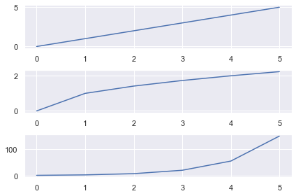
Matplotlib Subplots - A Helpful Illustrated Guide | Finxter

Excel charts: add title, customize chart axis, legend and data labels ... Click anywhere within your Excel chart, then click the Chart Elements button and check the Axis Titles box. If you want to display the title only for one axis, either horizontal or vertical, click the arrow next to Axis Titles and clear one of the boxes: Click the axis title box on the chart, and type the text.

How to Represent Data with a Pie of Pie Chart in Your Excel Worksheet - Data Recovery Blog

Add a DATA LABEL to ONE POINT on a chart in Excel Steps shown in the video above: Click on the chart line to add the data point to. All the data points will be highlighted. Click again on the single point that you want to add a data label to. Right-click and select ' Add data label ' This is the key step! Right-click again on the data point itself (not the label) and select ' Format data label '.

Share :