40 format data labels pane excel
How to Customize Your Excel Pivot Chart Data Labels - dummies Excel displays the Format Data Labels pane. Check the box that corresponds to the bit of pivot table or Excel table information that you want to use as the label. For example, if you want to label data markers with a pivot table chart using data series names, select the Series Name check box. How to Create Labels in Word from an Excel Spreadsheet - Online Tech Tips Select Browse in the pane on the right. Choose a folder to save your spreadsheet in, enter a name for your spreadsheet in the File name field, and select Save at the bottom of the window. Close the Excel window. Your Excel spreadsheet is now ready. 2. Configure Labels in Word.
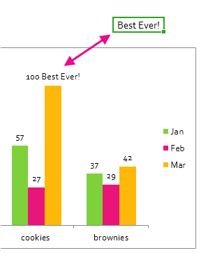
Add a DATA LABEL to ONE POINT on a chart in Excel You can now configure the label as required — select the content of the label (e.g. series name, category name, value, leader line), the position (right, left, above, below) in the Format Data Label pane/dialog box. To format the font, color and size of the label, now right-click on the label and select 'Font'. Note: in step 5. above, if ...
Format data labels pane excel
Excel data doesn't retain formatting in mail merge - Office Select File > Options. On the Advanced tab, go to the General section. Select the Confirm file format conversion on open check box, and then select OK. On the Mailings tab, select Start Mail Merge, and then select Step By Step Mail Merge Wizard. In the Mail Merge task pane, select the type of document that you want to work on, and then select Next. HOW TO STAGGER AXIS LABELS IN EXCEL - simplexCT Next, right-click the Series "+ label" Data Labels and then, on the shortcut menu, click Format Data Labels. 16. In the Format Data Labels pane, with Label Options selected, set the Label Position to Below. 17. Under Label Contains, click on Value Form Cells. In the Data Label Range dialog box set the Select Data Label Range to refer to B3:B11. Excel 2016 Tutorial Formatting Data Labels Microsoft Training Lesson FREE Course! Click: about Formatting Data Labels in Microsoft Excel at . A clip from Mastering Excel M...
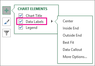
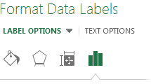
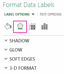
Format data labels pane excel. Format Data Label: Label Position - Microsoft Community when you add labels with the + button next to the chart, you can set the label position. In a stacked column chart the options look like this: For a clustered column chart, there is an additional option for "Outside End" When you select the labels and open the formatting pane, the label position is in the series format section. Does that help? Excel Charts - Aesthetic Data Labels - tutorialspoint.com To format the data labels − Step 1 − Right-click a data label and then click Format Data Label. The Format Pane - Format Data Label appears. Step 2 − Click the Fill & Line icon. The options for Fill and Line appear below it. Step 3 − Under FILL, Click Solid Fill and choose the color. Change the format of data labels in a chart To get there, after adding your data labels, select the data label to format, and then click Chart Elements > Data Labels > More Options. To go to the appropriate area, click one of the four icons ( Fill & Line, Effects, Size & Properties ( Layout & Properties in Outlook or Word), or Label Options) shown here. How to add data labels from different column in an Excel chart? In the Format Data Labels pane, under Label Options tab, check the Value From Cells option, select the specified column in the popping out dialog, and click the OK button. Now the cell values are added before original data labels in bulk. 4. Go ahead to untick the Y Value option (under the Label Options tab) in the Format Data Labels pane.
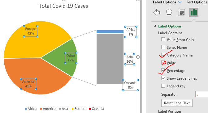
Formatting data labels and printing pie charts on Excel for Mac 2019 ... Here's a work around I found for printing pie charts. Still can't find a solution for formatting the data labels. 1. When printing a pie chart from Excel for mac 2019, MS instructions are to select the chart only, on the worksheet > file > print. Excel is supposed to print the chart only (not the data ) and automatically fit it onto one page. Excel Pie Chart - How to Create & Customize? (Top 5 Types) Step 1: Click on the Pie Chart > click the ' + ' icon > check/tick the " Data Labels " checkbox in the " Chart Element " box > select the " Data Labels " right arrow > select the " More Options… ", as shown below. Step 2: The Format Data Labels pane opens. Go to the " Label Options ", and check/tick the " Percentage ... How to Print Labels from Excel - Lifewire Select Mailings > Write & Insert Fields > Update Labels . Once you have the Excel spreadsheet and the Word document set up, you can merge the information and print your labels. Click Finish & Merge in the Finish group on the Mailings tab. Click Edit Individual Documents to preview how your printed labels will appear. Select All > OK . How to Create Mailing Labels in Excel | Excelchat Step 1 - Prepare Address list for making labels in Excel First, we will enter the headings for our list in the manner as seen below. First Name Last Name Street Address City State ZIP Code Figure 2 - Headers for mail merge Tip: Rather than create a single name column, split into small pieces for title, first name, middle name, last name.
How to format axis labels as thousands/millions in Excel? - ExtendOffice Right click at the axis you want to format its labels as thousands/millions, select Format Axisin the context menu. 2. In the Format Axisdialog/pane, click Number tab, then in theCategorylist box, select Custom, and type[>999999] #,,"M";#,"K"into Format Codetext box, and click Addbutton to add it toTypelist. See screenshot: 3. Format Chart Axis in Excel - Axis Options Analyzing Format Axis Pane. Right-click on the Vertical Axis of this chart and select the "Format Axis" option from the shortcut menu. This will open up the format axis pane at the right of your excel interface. Thereafter, Axis options and Text options are the two sub panes of the format axis pane. Format Data Labels in Excel- Instructions - TeachUcomp, Inc. To do this, click the "Format" tab within the "Chart Tools" contextual tab in the Ribbon. Then select the data labels to format from the "Chart Elements" drop-down in the "Current Selection" button group. Then click the "Format Selection" button that appears below the drop-down menu in the same area. Add or remove data labels in a chart - support.microsoft.com Right-click the data series or data label to display more data for, and then click Format Data Labels. Click Label Options and under Label Contains, select the Values From Cells checkbox. When the Data Label Range dialog box appears, go back to the spreadsheet and select the range for which you want the cell values to display as data labels.
Add or remove data labels in a chart
How to Add Data Labels to an Excel 2010 Chart - dummies On the Chart Tools Layout tab, click Data Labels→More Data Label Options. The Format Data Labels dialog box appears. You can use the options on the Label Options, Number, Fill, Border Color, Border Styles, Shadow, Glow and Soft Edges, 3-D Format, and Alignment tabs to customize the appearance and position of the data labels.
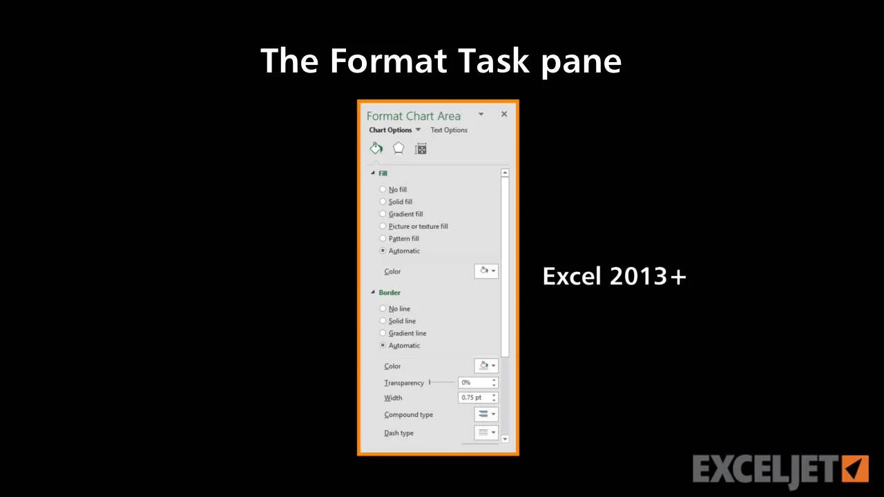
The Format Task pane
Excel Charts - Quick Formatting - tutorialspoint.com The Format pane by default appears on the right-side of the chart. Step 1 − Click on the chart. Step 2 − Right-click the horizontal axis. A drop-down list appears. Step 3 − Click Format Axis. The Format pane for formatting axis appears. The format pane contains the task pane options. Step 4 − Click the Task Pane Options icon.
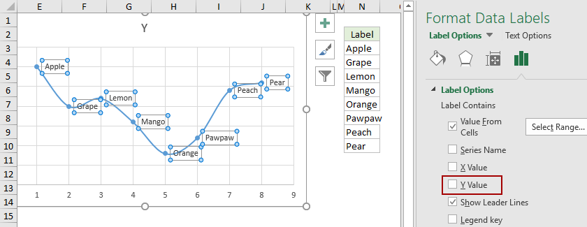
How to add data labels from different column in an Excel chart?
2/ Right-click i.e. on the 1st histo. bar (A) > Add Data Labels (numbers are displayed a the top of the bars) 3/ Click one of the numbers that just displayed (the Format Data Labels pane opens on the right) > Check option "Value From Cells" > Select range C2:C7 > OK > Uncheck option "Value" demo.png(18.5 KiB) Comment Comment ·

Add a Data Callout Label to Charts in Excel 2013 – Software ...
How to Print Labels From Excel - EDUCBA Navigate towards the folder where the excel file is stored in the Select Data Source pop-up window. Select the file in which the labels are stored and click Open. A new pop up box named Confirm Data Source will appear. Click on OK to let the system know that you want to use the data source. Again a pop-up window named Select Table will appear.

Adding rich data labels to charts in Excel 2013 | Microsoft ...
Excel tutorial: The Format Task pane You can also select a chart element first, then use the keyboard shortcut Control + 1. For example, if I select the data bars in this chart, then type Control + 1, the Format Task Pane will open with with the data series options selected. The Format Task pane stays open until you manually close the window.
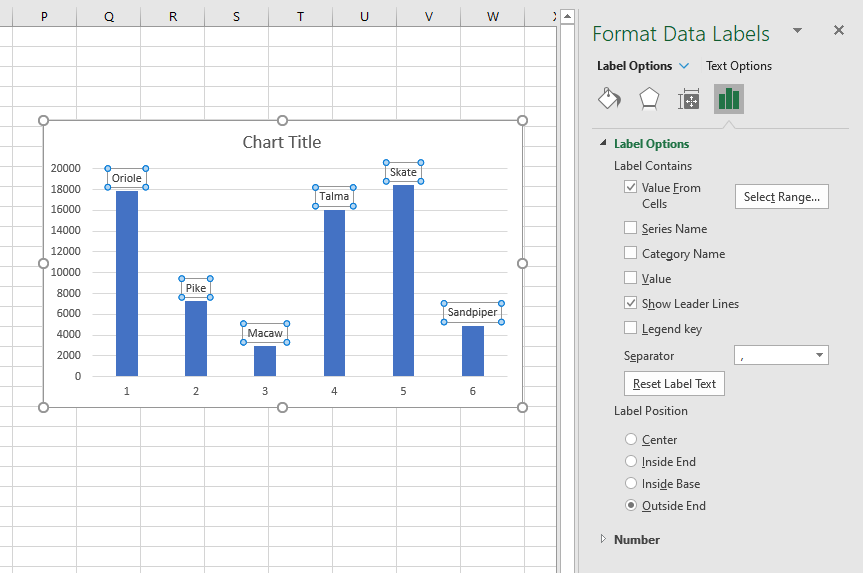
Custom data labels in a chart
Stagger long axis labels and make one label stand out in an Excel ... The method also involves forcing Excel to use every label and trick it by rotating the labels and then rotating them back. If all you need to do is to stagger the labels, use this method. ... Add Data Labels using the "+" chart skittle and navigate to the More Options selection to open the Format Data Labels task pane. In the Label Options ...
Change the format of data labels in a chart
How to Add Data Labels to Scatter Plot in Excel (2 Easy Ways) - ExcelDemy From the drop-down list, select Data Labels. After that, click on More Data Label Options from the choices. By our previous action, a task pane named Format Data Labels opens. Firstly, click on the Label Options icon. In the Label Options, check the box of Value From Cells.
Dynamically Label Excel Chart Series Lines • My Online ...
Pie Chart in Excel - Inserting, Formatting, Filters, Data Labels Click on the Instagram slice of the pie chart to select the instagram. Go to format tab. (optional step) In the Current Selection group, choose data series "hours". This will select all the slices of pie chart. Click on Format Selection Button. As a result, the Format Data Point pane opens.
Change the format of data labels in a chart
How do you format data series in Excel? - FAQ-ALL To format data labels in EÎl , choose the set of data labels to format . To do this, click the " Format " tab within the "Chart Tools" contextual tab in the Ribbon. Then select the data labels to format from the "Chart Elements" drop-down in the "Current Selection" button group. How do I show the Format Data Series pane in Excel?
Using the CONCAT function to create custom data labels for an ...
Excel tutorial: How to use data labels When first enabled, data labels will show only values, but the Label Options area in the format task pane offers many other settings. You can set data labels to show the category name, the series name, and even values from cells. In this case for example, I can display comments from column E using the "value from cells" option.
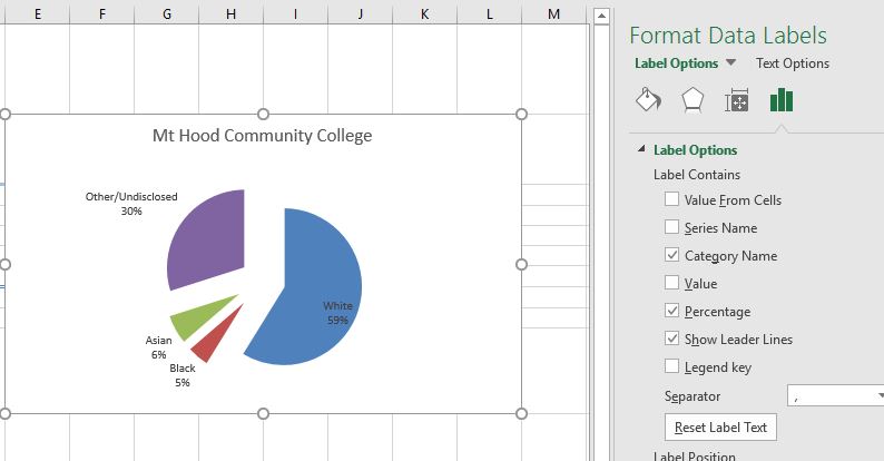
4.1.3 Choosing a Chart Type: Pie Chart – Excel For Decision ...
Excel 2016 Tutorial Formatting Data Labels Microsoft Training Lesson FREE Course! Click: about Formatting Data Labels in Microsoft Excel at . A clip from Mastering Excel M...
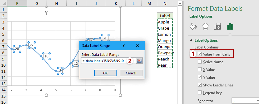
How to add data labels from different column in an Excel chart?
HOW TO STAGGER AXIS LABELS IN EXCEL - simplexCT Next, right-click the Series "+ label" Data Labels and then, on the shortcut menu, click Format Data Labels. 16. In the Format Data Labels pane, with Label Options selected, set the Label Position to Below. 17. Under Label Contains, click on Value Form Cells. In the Data Label Range dialog box set the Select Data Label Range to refer to B3:B11.

Adding rich data labels to charts in Excel 2013 | Microsoft ...
Excel data doesn't retain formatting in mail merge - Office Select File > Options. On the Advanced tab, go to the General section. Select the Confirm file format conversion on open check box, and then select OK. On the Mailings tab, select Start Mail Merge, and then select Step By Step Mail Merge Wizard. In the Mail Merge task pane, select the type of document that you want to work on, and then select Next.
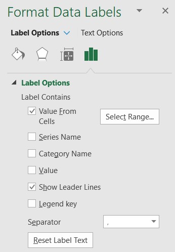
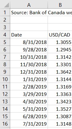
Using the CONCAT function to create custom data labels for an ...
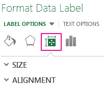
Change the format of data labels in a chart
Change the format of data labels in a chart

How to show percentages on three different charts in Excel ...

How to add labels to the Marimekko chart - Microsoft Excel 365
How to Rotate Data Labels in Excel (2 Simple Methods)
When to Use Bar of Pie Chart in Excel

How to improve or conditionally format data labels in Power ...
Change the format of data labels in a chart
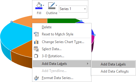
Excel 3-D Pie charts - Microsoft Excel 2016
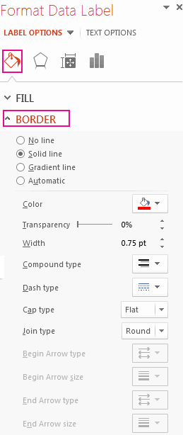
Change the format of data labels in a chart
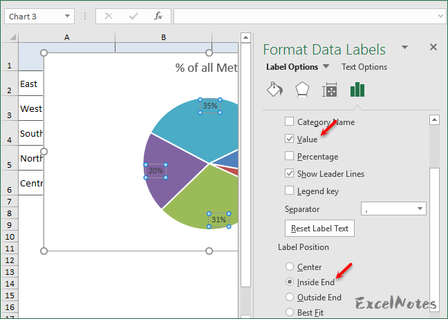
How to Make Pie Chart with Labels both Inside and Outside ...
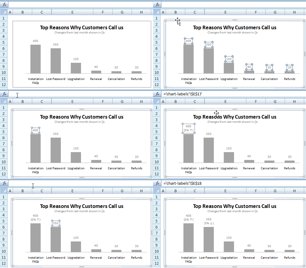
How to Change Excel Chart Data Labels to Custom Values?
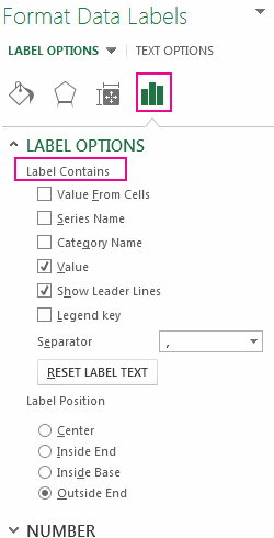
Add or remove data labels in a chart
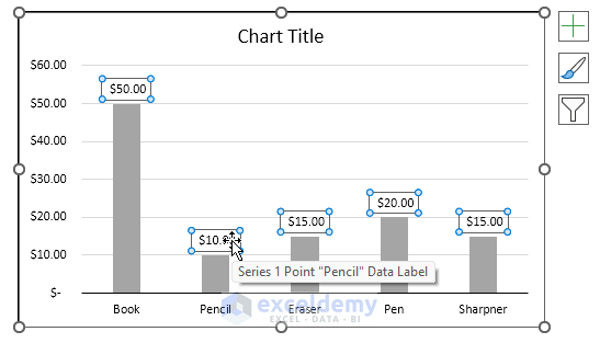
How to Move Data Labels In Excel Chart (2 Easy Methods)
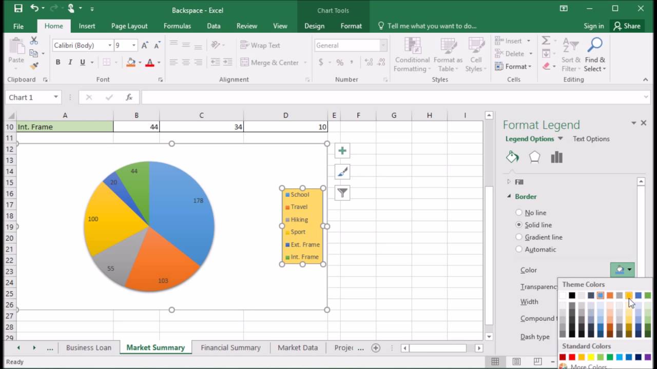
409 How to use Format pane to format the chart legend in Excel 2016
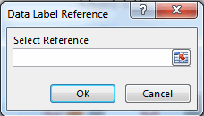
Change the format of data labels in a chart
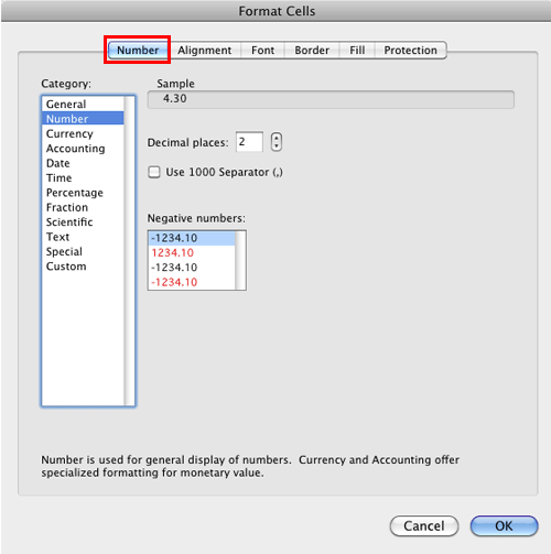
Format Number Options for Chart Data Labels in Excel 2011 for Mac
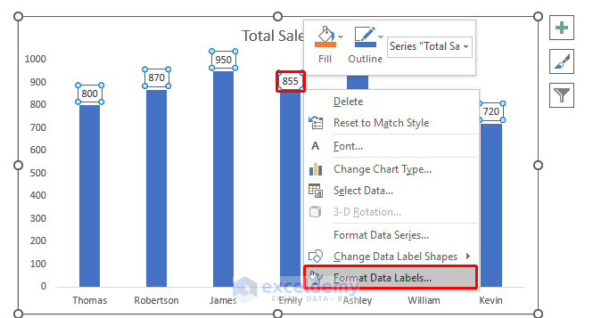
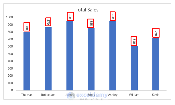
How to Rotate Data Labels in Excel (2 Simple Methods)
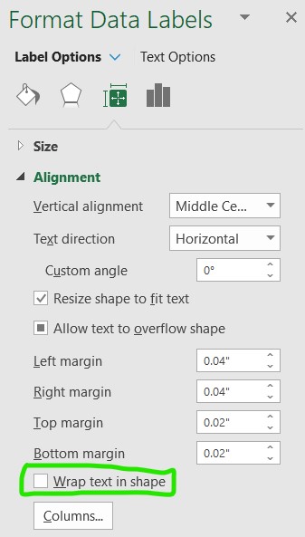
Stagger long axis labels and make one label stand out in an ...
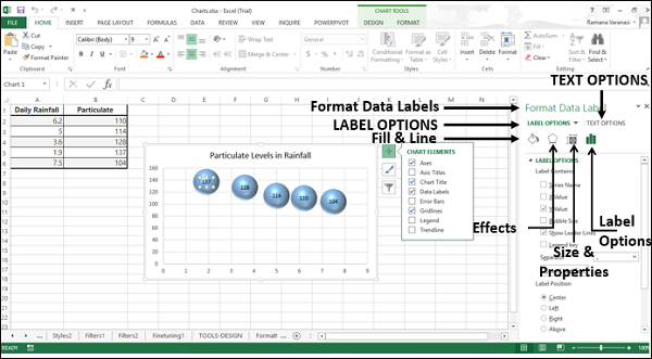
Excel Charts - Aesthetic Data Labels
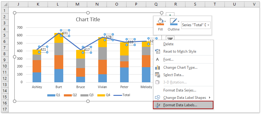
How to add total labels to stacked column chart in Excel?
How to add a text label in the chart of MS Excel - Quora

Format Data Labels in Excel- Instructions - TeachUcomp, Inc.
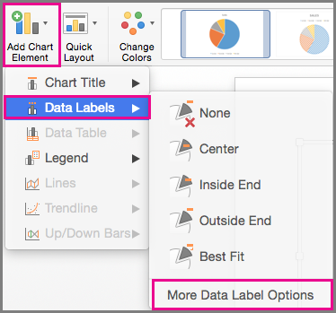
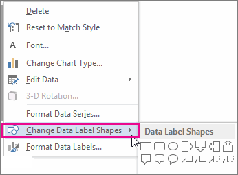
Change the format of data labels in a chart
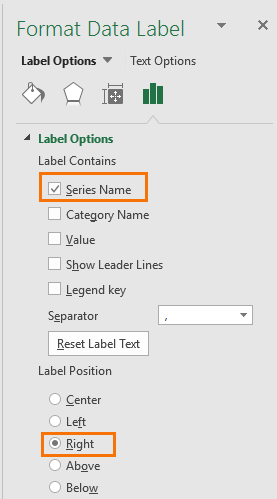
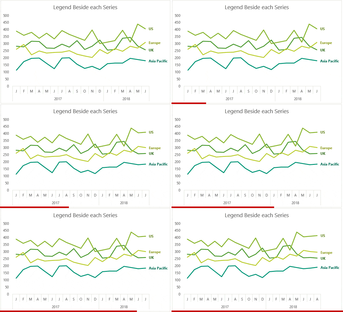
Dynamically Label Excel Chart Series Lines • My Online ...

How to Make a PIE Chart in Excel (Easy Step-by-Step Guide)
Post a Comment for "40 format data labels pane excel"